Target Audience: Data Scientists
Introduction
Kafka. Flink. Debezium. Materialize. These are a small sampling of streaming data tools you may have heard of recently. They make up components of the real-time data stack, a specialized set of tools for working with continuous streams of data and reacting to them in milliseconds.
Real-time data isn’t new. We’ve had real-time data sources and associated services for decades. But the tools & techniques were cumbersome and expensive in the past, which kept deployment of real-time data stacks limited to niche, high value use cases (energy, finance, fraud detection, etc).
What’s different now?
We have 3 key trends that all reinforce each other:
- an exponential rise the real-time data generation capacity in all industries (e.g. energy, finance, and supply chain)
- a proliferation of real-time goods & services that work with those data feeds (on-demand taxis, real-time flight gate changes, etc)
- expectations of customers globally of real-time experiences (accurate food delivery ETAs, real-time location updates of couriers, etc)
Working with continuous incoming data presents unique technical challenges, but the current generation of tooling has made working with real-time data streams extremely accessible. A single data scientist can now build and deploy scalable streaming workflows in just an afternoon.
Learning Overview
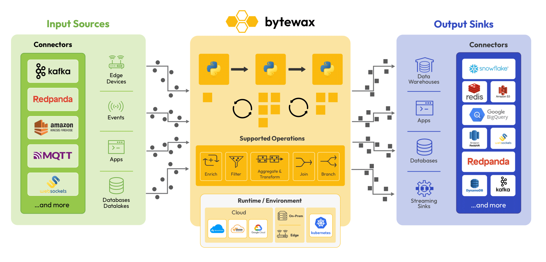
In this series, we’ll teach you all of the concepts and tools you need to know to build real-time data pipelines entirely in Python and SQL. Most of this series will be taught using the Bytewax library, our open-source Python library for stream processing.
No previous experience with streaming data, the Bytewax library, or other languages (like Java) is necessary to thrive in this series. This hands-on tutorial is split into 4 parts:
- Part I: Foundational Concepts for Stream Data Processing
- Part II: Controlling Time with Windowing & Sessionization
- Part III: Joining Streams
- Part IV: Real-time Machine Learning
First Principles Terminology
Before diving into code and data processing logic, I want to start by providing some context into the basic concepts and terminology that I think is essential.
Real-time
What is a real-time data system? Real-time systems aspire to some type of latency guarantee that’s usually sub-second (1 to 1,000 milliseconds). Working with real-time data means that you’re operating in the low latency arena.
- When you swipe a credit card at a coffee shop, many steps have to occur to validate and authorize the payment. No coffee shop or coffee customer wants to wait really more than a few seconds for the entire process to magically work behind the scenes. This means that most of the important steps like fraud detection need to happen in milliseconds, not seconds.
- High frequency trading systems respond to market signals and make trade requests in just a few milliseconds. Designing a profitable system here requires a strong command of latency throughout the entire system.
Streaming Data
In the excellent Streaming 101 article, Tyler Akaidu renames “streaming data” to unbounded data:
- Unbounded data: A type of ever-growing, essentially infinite data set. These are often referred to as “streaming data.” However, the terms streaming or batch are problematic when applied to data sets, because as noted above, they imply the use of a certain type of execution engine for processing those data sets. The key distinction between the two types of datasets are tied to their execution because of the knowledge of whether there is a known end to the data. In this article, I will refer to infinite “streaming” data sets as unbounded data, and finite “batch” data sets as bounded data.
Instead of trying to craft our own explanation, we’re adopting Tyler Akidau's excellent framing here. A stream of data refers to an unbounded set of incoming data points.
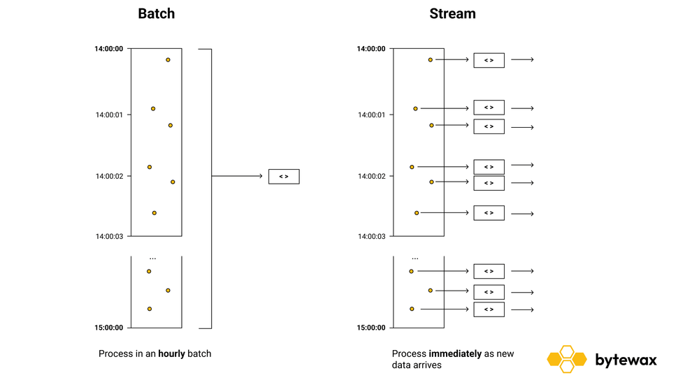
Batch vs Stream Processing
Batch Processing
Batch processing involves handling & processing data in a pre-defined schedule (every hour, day, etc) or in pre-defined chunks (every 1 MB, 1 GB, etc) of data. Batch processing is the most popular approach in most organizations because they excel at handling large volumes of data and low latency isn’t important for many use cases (especially internal data analysis).
- If you only validate credit card payments once a minute, then more than 90% of your customers will not be able to pay for coffee in seconds. Batch systems don’t operate in the low latency arena.
Stream Processing
Stream processing involves handling data continuously as it arrives. With this approach, we can react and operate in the sub-second scale as long as we maintain this low-latency requirement through the next stages of our data pipeline as well.
In batch processing, time or batches of data are pre-defined and scheduled. Because everything is immediate and reactive in stream processing workloads, time is given back to the data scientist or data engineer to control as they see fit.
- When validating credit card payments, we can design our system to react as quickly as possible.
- For certain types of calculations (e.g. minutely or hourly metrics), we can maintain the running state and gradually mirror the batch processing workflow only when we need it.
Generators & Iterators
To get comfortable quickly with basic streaming concepts, we’ll start by exploring them using native Python concepts like generators and iterators before moving onto building stream processing workflows in Bytewax.
The following code defines the rand_stream() function, which generates a random integer between 0 and 100 until the control flow is uninterrupted (while True). We can use this to simulate generating an unlimited stream of values. To simulate how a consume would interact with the stream, we yield the value to make this a generator function, which is very common in client libraries for streaming data.
# Generator
import random
import time

def rand_stream():
  while True:
    i = random.randint(0, 100)
    yield i
To consume from the stream, we can use the iterator tools available object to request values from the generator.
print(next(rand_stream()))
>> 3

for r in iter(rand_stream()):
    print(r)
    # Adding so output slowly prints
    time.sleep(0.25)

>> 95
>> 55
>> 9
...
We can use this to simulate a simple real-world stream of incoming data for us to process.
Mapping Values
When you receive a stream of events, you often want to apply some simple transformation to ALL events. Here are some examples:
- Convert values to a particular datetime format
- Enriching an object with additional metadata
- Masking sensitive account information
In vanilla Python, we’d use the map() function to accomplish this. The following code applies the same transformation to all values from the generator we created earlier:
mapped_values = list(map(lambda x: x * 2, rand_stream))
Filtering Values
What if we instead want to apply a transformation to just a subset of the values we’re receiving? We can use filter for this.
less_than_fifty = list(filter(lambda x: x < 50, mapped_values))
Streaming Workflows
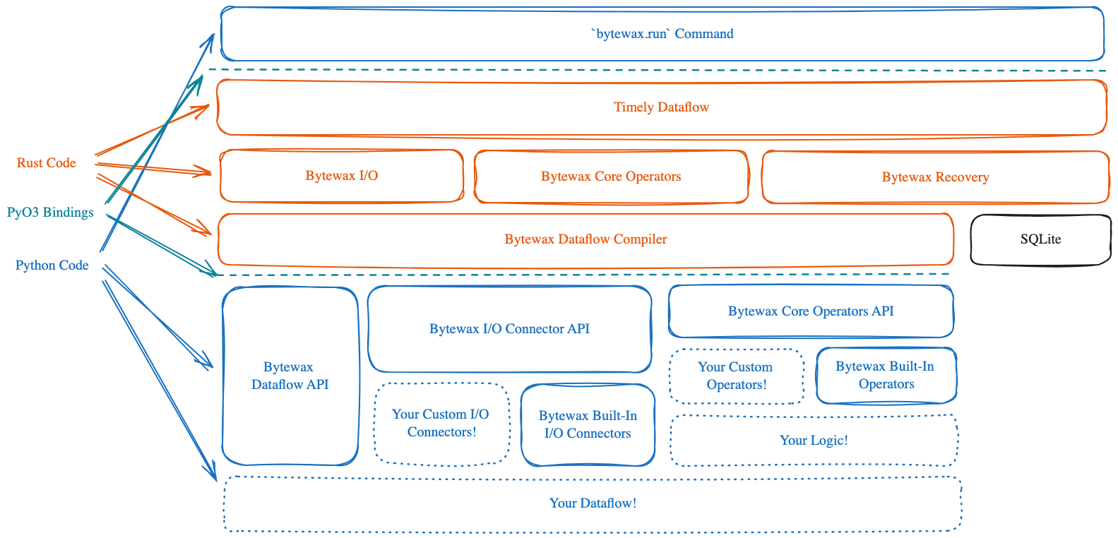
Bytewax, as well as other stream processing frameworks, are designed around a workflow centric approach. More specifically, Bytewax takes a dataflow approach to running workloads which means that your code is compiled into a DAG (directed acyclic graph) for the underlying engine to run. This bakes in a helpful separation of concerns:
- data scientists and data engineers can write short Pythonic workflows to perform complex stream procesisng calculations
- infrastructure engineers (as well as contributors to the bytewax library) focus on adding support for fault tolerance, monitoring, workflow visualization, and scalability to more nodes
As the data scientist or data engineer creating bytewax dataflow jobs, you thankfully don’t have to understand the implementation details under the hood (the red parts of the diagram below).
When you define a streaming workflow, it’s important to know the difference between stateless and stateful operations.
Stateless Operations
Mapping and filter values are both considered stateless operations because every incoming data point in the stream is handled and resolved without any dependencies between datapoints or delays in processing. As mentioned in our docs, stateless operations only operate on individual items and forget all context between them.
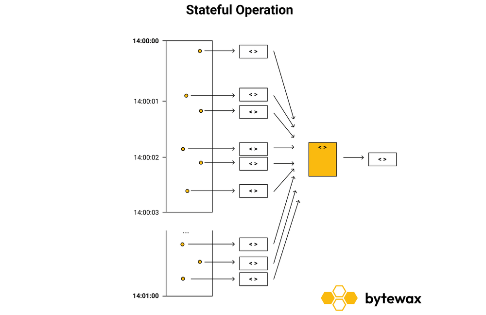
Stateful Operations
Aggregations, on the other hand, require the maintenance of intermediate state until your pre-defined criteria is met and the computed aggregate is “released” into the next step in your workflow. Here are some examples where stateful operations are needed:
- Calculate a minute-level average of temperature from incoming temperature signals
- Collect all events (state) in a 60 second period and average them
- Calculate the likelihood that a payment transaction is fraudulent or not
- Collect events from multiple streams (over a few miliseconds) of data and apply a previuosly trained fraud model
The diagram below highlights how a window of one minute would collect all of the events into a single collection that can then be analyzed or reduced further.
Bytewax Introduction
We’re now ready to build our first stream processing workflow in Bytewax! This workflow will operate on a bounded set of data (all the words in our text file) so we can speed up the learning process and reduce the friction to experiment. We’ll remove this limitation later in the series when we connect it to a real, unbounded stream of data.
We will use some of the ideas previously discussed. Stateless operations can be used to modify each word in the text file and stateful operations can be used to count the words in the text file incrementally.
- Start by installing bytewax:
pip install bytewax
- Create a file called wordcount.py and paste in the following page of code:
import operator
import re
from datetime import timedelta, datetime, timezone

from bytewax.dataflow import Dataflow
import bytewax.operators as op
from bytewax.connectors.files import FileSource
from bytewax.connectors.stdio import StdOutSink

flow = Dataflow("wordcount_eg")
inp = op.input("inp", flow, FileSource("wordcount.txt"))

def lower(line):
    return line.lower()

lowers = op.map("lowercase_words", inp, lower)

def tokenize(line):
    return re.findall(r'[^\s!,.?":;0-9]+', line)

tokens = op.flat_map("tokenize_input", lowers, tokenize)
counts = op.count_final("count", tokens, lambda word: word)

op.output("out", counts, StdOutSink())
Let’s walk through the steps in this Bytewax dataflow
- The code snippet below instantiates a new Dataflow object. This object acts as a "container" for all the steps in our dataflow.
flow = Dataflow("wordcount_eg")
- The next line adds the FileSource connector as an input named inp to the pipeline. This connector reads in any text file line-by-line.
inp = op.input("inp", flow, FileSource("wordcount.txt"))
- Next we use a
lower()function in amap()operator step named lowercase_words. This operator applies a mapper function (in our caselower()) to every upstream item (line of text).
def lower(line):
    return line.lower()

lowers = op.map("lowercase_words", inp, lower)
- Then the
tokenize()function is used to split up a line of text into individual words using a regular expression when called in aflat_mapstep named tokenize_input that takes inlowersas an input and emits an output of every transformed word.
def tokenize(line):
    return re.findall(r'[^\s!,.?":;0-9]+', line)

tokens = op.flat_map("tokenize_input", lowers, tokenize)
- The next step adds a stateful
count_final()step that collects all of the words (tokens) and counts them.
counts = op.count_final("count", tokens, lambda word: word)
- Finally outputs the resulting word counts to standard out using the
StdOutSink()sink.
op.output("out", counts, StdOutSink())
This is the result when we run this program.
> python -m bytewax.run wordcount
("'tis", 1)
('a', 1)
('against', 1)
('and', 2)
('arms', 1)
('arrows', 1)
('be', 2)
('by', 1)
('end', 1)
('fortune', 1)
('in', 1)
('is', 1)
('mind', 1)
('nobler', 1)
('not', 1)
('of', 2)
('opposing', 1)
('or', 2)
('outrageous', 1)
('question', 1)
('sea', 1)
('slings', 1)
('suffer', 1)
('take', 1)
('that', 1)
('the', 3)
('them', 1)
('to', 4)
('troubles', 1)
('whether', 1)
Up Next
Next, in part 2, we will dig into the concept of windows and sessionization, crucial aspects to understand while working with streaming data.
That's a wrap on part 1 of this series. We hope you enjoyed it! If you have some questions or want to give us some feedback drop into 🐝 slack or send us an email!
Want to see more Bytewax in action - check out our guides for some complete examples.
Choosing the Right Streaming Platform: Kafka vs. Pulsar vs. NATS

Zander Matheson
CEO, FounderZander is a seasoned data engineer who has founded and currently helms Bytewax. Zander has worked in the data space since 2014 at Heroku, GitHub, and an NLP startup. Before that, he attended business school at the UT Austin and HEC Paris in Europe.